
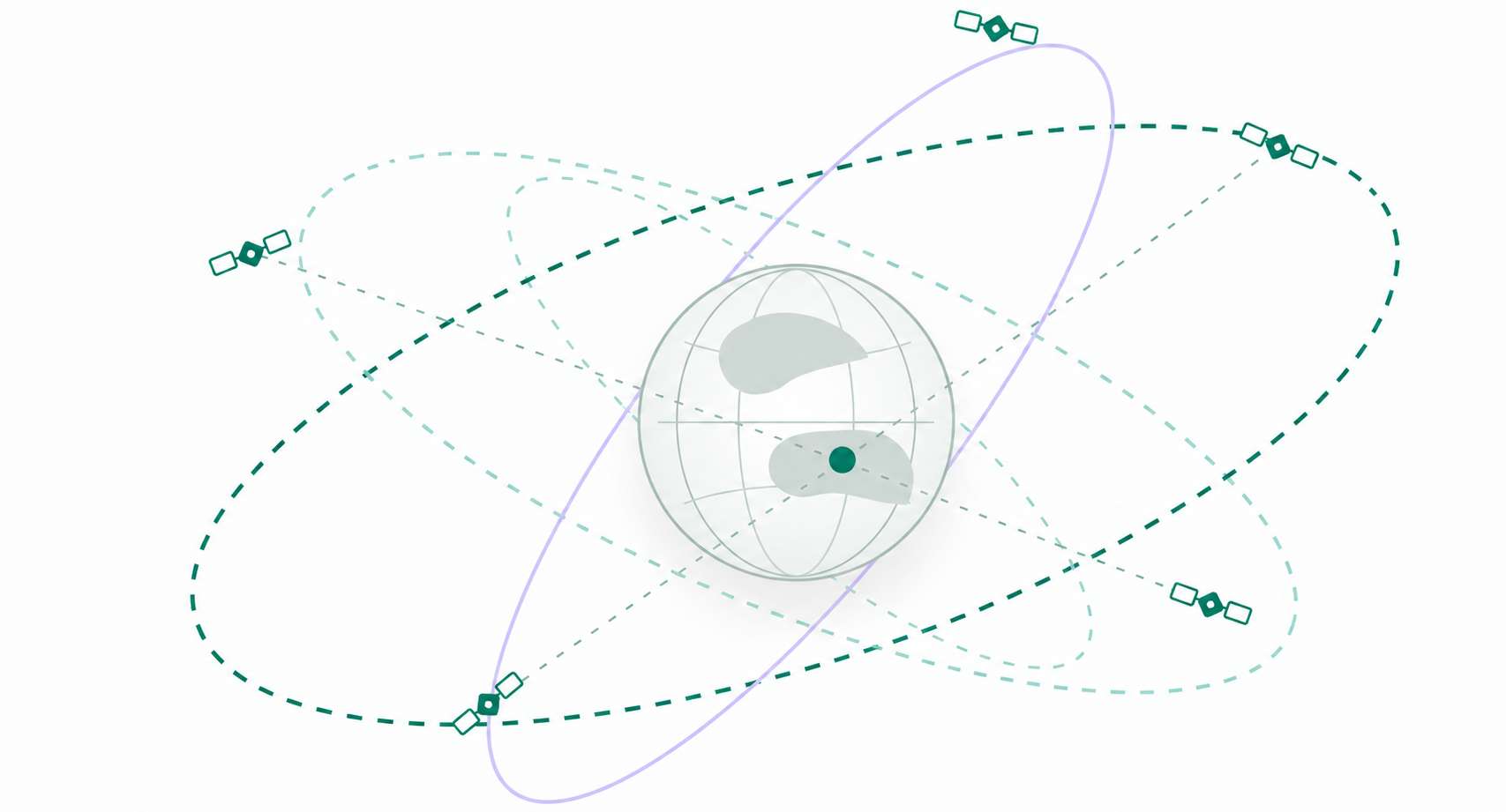
Tutorial overview
Numbers before abstraction
This tutorial builds a Single Point Positioning (SPP) solution from first principles using only code pseudorange observations and broadcast ephemeris. Each formula is paired with real numbers so you can see exactly how results are obtained.
- Derive the measurement model and apply key corrections
- Linearize and solve the system with weighted least squares
- Iterate to obtain the receiver position and clock bias
- Validate the solution and understand common pitfalls
What you build
A clear, modular SPP pipeline you can implement in Python, MATLAB, or C++.
Processing pipeline
From code ranges to receiver position
RINEX observations
Raw pseudorange measurements
Satellite position & clock
Broadcast ephemeris + clock model
Earth rotation correction
Sagnac effect applied
Atmospheric corrections
Ionosphere & troposphere
Linearized model
Observation equation
Weighted least squares
Solve for state update
Receiver position
Iterate to convergence
Selected inputs
Raw observations and selected satellite
RINEX snippet
Raw observation epoch
| SV | Pseudorange (m) | Elevation | Azimuth | SNR |
|---|---|---|---|---|
| G09 | 20,149,603.512 | 74.43 deg | 55.08 deg | not exported |
| G07 | 21,134,422.504 | 65.60 deg | 307.44 deg | not exported |
| G04 | 21,325,674.301 | 47.10 deg | 99.20 deg | not exported |
| G30 | 22,518,702.199 | 36.90 deg | 268.55 deg | not exported |
| G16 | 23,464,421.180 | 19.60 deg | 42.58 deg | not exported |
Broadcast ephemeris
G09 compact row
Toe
378,000 s
t_tx
377,999.932345 s
sat clock
4.430247e-4 s
more parameters
NAV record
Elevation
74.43 deg
Azimuth
55.08 deg
Checkpoint 1
Worked numerical arc (G09) - Pseudorange model
P_corr = 20,149,603.512 - c*dt_s - Sagnac + I + T
P_corr = 20,149,603.512 + -132,815.465 - -5.640 + 9.999 + 0.000
P_corr = 20,282,408.839 m
residual = 20,282,408.839 - 20,282,408.337
Modeled/corrected
20,282,408.839 m
Measured raw
20,149,603.512 m
Pre-fit residual
0.502 m
Core corrections
Transmit-time estimation and corrected range
From raw observations to a corrected geometric range. Each correction is computed numerically so you can see how meters are gained or lost before solving for position.
Transmit time
Satellite clock correction
Broadcast ephemeris snippet
RINEX navigation record
G09 2024 11 14 10 00 00  4.430247051307D-04
     toe = 378000.000 s       sqrtA/e/i0 exported in NAV
     t_tx = 377999.932345 s   delta_t_s = 4.430247051307D-04 s
     Sagnac = -5.639826 m     I_L1 = 9.999084 m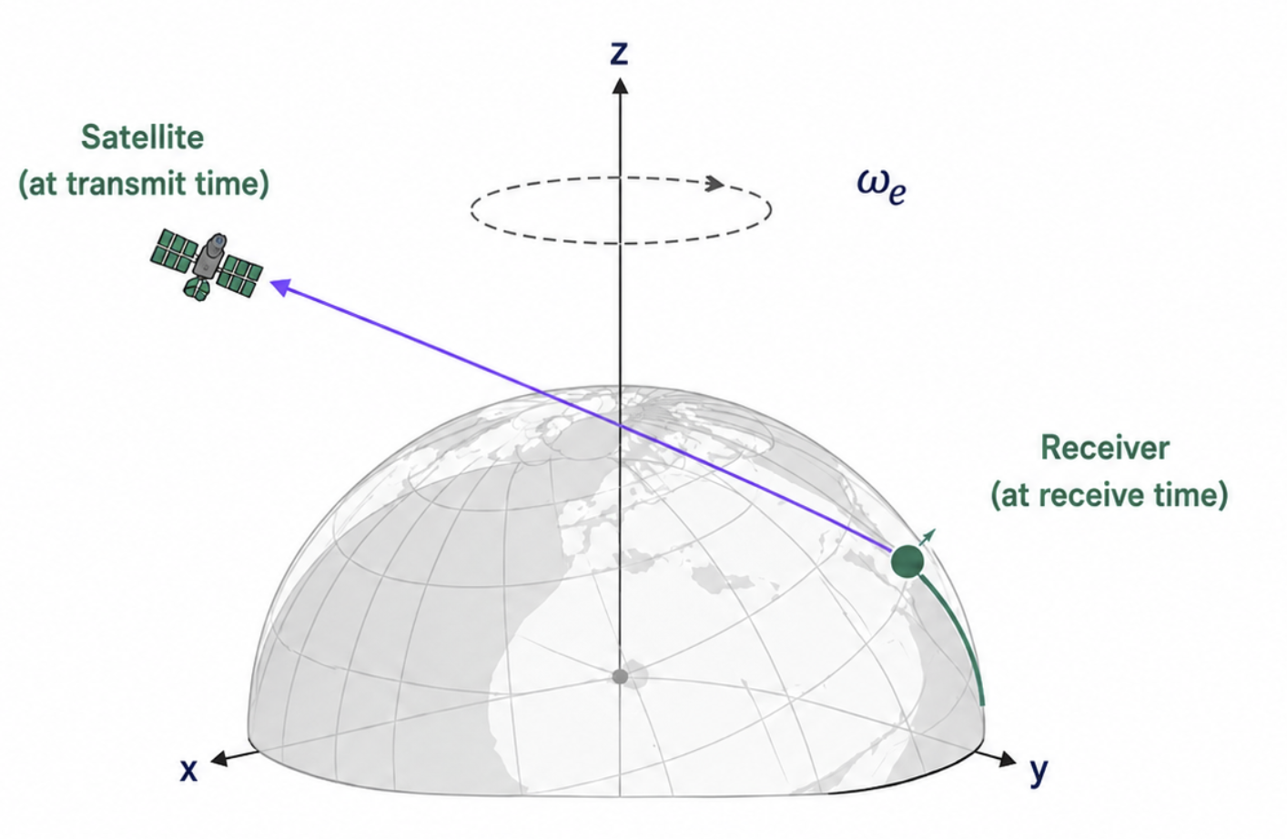
Earth rotation / Sagnac
Ionosphere correction
Klobuchar model correction
Troposphere correction
Troposphere model correction
Numerical checkpoint
Corrected geometric range
rho_corr = 20,149,603.512 + -132,815.465 - (-5.640) + 9.999 + 0.000
rho_corr = 20,282,408.839 m
Summary of corrections
Linearized measurement model
Turn corrected ranges into a solvable system
State correction vector
Design matrix
Bias/correction vector
delta rho: observation residuals. b: modeled corrections. epsilon: measurement noise.
Geometry insight
Design matrix row and geometric residual (G09)
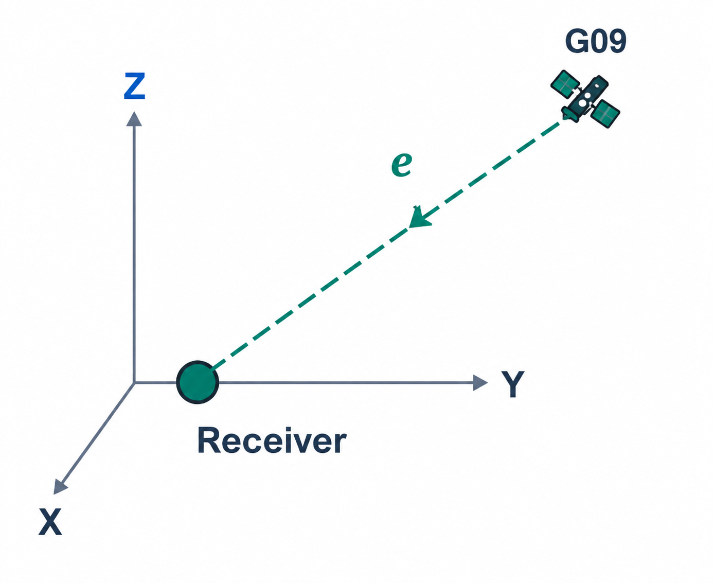
Design matrix row
Geometric range
Geometric residual
0.5021 m
Build all satellite rows
Every satellite becomes one row of H
| SV | Elev | Pseudorange corrected | Geometric range | Residual | Design matrix row A_s |
|---|---|---|---|---|---|
| G09 | 74.43 | 20,282,408.839 | 20,282,408.337 | 0.5021 | [-0.2633, -0.6808, -0.6835, 1.0000] |
| G07 | 65.60 | 21,128,343.944 | 21,128,344.609 | -0.6655 | [-0.6290, -0.2606, -0.7324, 1.0000] |
| G04 | 47.10 | 21,469,331.005 | 21,469,331.378 | -0.3731 | [0.1118, -0.9352, -0.3359, 1.0000] |
| G30 | 36.90 | 22,434,075.292 | 22,434,075.198 | 0.0939 | [-0.9372, 0.1088, -0.3315, 1.0000] |
| G16 | 19.60 | 23,425,789.901 | 23,425,789.970 | -0.0691 | [0.5779, -0.2982, -0.7597, 1.0000] |
Pre-fit residuals
m
5
mean
-0.102 m
RMS
0.412 m
Weighted least squares
Solve the linearized system
Solution (this iteration)
Iteration 1
Delta x
-17.9810 m
Delta y
17.9596 m
Delta z
5.5403 m
Delta cdt
-0.1023 m
Position update norm
26.0108 m
Satellites used
5
Solve and iterate
Repeat until the update collapses
Form linearized model
Build H and Delta rho
Weighted least squares
Compute Delta theta
Update state
Check convergence
Position & clock norms
Repeat until solved
Thresholds met
Final iteration
2
Position update
0.00009981 m
RMS post-fit
0.398870 m
Converged
Yes
Quality checks
Residual diagnostics, DOP, and matrix structure
Iteration history
| it | update | RMS | clock |
|---|---|---|---|
| 1 | 26.010765 | 0.398873 | -0.102312 |
| 2 | 0.000100 | 0.398870 | -0.102321 |
Convergence chart
Converged at iteration 2.
Post-fit residuals
All residuals are within +/-1 m in this exported solution.
DOP summary
GDOP
3.69
PDOP
3.15
HDOP
2.12
VDOP
2.34
TDOP
1.93
Design matrix heatmap
Prefit to postfit check
Worked example summary
Final SPP solution
ECEF position
X
3,246,356.6055 m
Y
4,052,683.3535 m
Z
3,693,181.6012 m
Geodetic
Latitude
35.60388432 deg
Longitude
51.30391819 deg
Height
1,092.738 m
Metrics
RMS post-fit
0.398870 m
PDOP
3.153
Used satellites
5
Model
code
SPP solution complete
You built this
Receiver position from pseudorange observations
You successfully computed a GNSS receiver position from pseudorange observations using Single Point Positioning. Next up: examine DOP and error sources, then build a carrier-phase relative-positioning model with double differences.

Continue your learning
Next numerical threads
DOP and Geometry
Understand GDOP, PDOP and satellite geometry
OpenError Sources in GNSS
Ionosphere, troposphere, multipath and more
OpenLAMBDA Ambiguity Resolution
Search integer ambiguities using covariance and decorrelation
OpenDouble Difference Positioning
Build a correlated carrier-phase model from real RINEX data
OpenReal Data Walkthroughs
RINEX examples and case studies
Open