LAMBDA Method for GNSS Integer Ambiguity Resolution

Tutorial overview

Numbers before abstraction

What LAMBDA solves

Least squares gives real-valued ambiguity estimates, but carrier-phase ambiguities are integers. LAMBDA uses their covariance to search for the integer vector that best fits the complete statistical model.

Teaching pattern

Formula -> values -> arithmetic -> result

The same compact sequence repeats through every numerical checkpoint.

1

Float ambiguities

Estimate real-valued ambiguities and covariance

2

Integer least squares

Define the covariance-weighted search

3

Decorrelate

Transform into a search-friendly integer space

4

Search

Find the two best integer candidates

5

Back-transform

Return candidates to the original order

6

Compare

Rank candidates and report diagnostics

1. Carrier-phase ambiguity

Why ambiguity fixing matters

A carrier-phase ambiguity is an unknown whole number of carrier cycles. The physical truth belongs to the integers, but measurement noise and least-squares estimation first produce a real-valued float estimate.

Integer truth

\mathbf N\in\mathbb Z^n

Float estimate

\hat{\mathbf a}\in\mathbb R^n

1Integer truth

2Measurements + least squares

3Float ambiguity estimate

4Integer search

2. Real Qelora input

Float ambiguities and their covariance

Float ambiguity vector

\hat{\mathbf a}=\begin{bmatrix}1.23\\5.78\\-2.41\end{bmatrix}\;\mathrm{cycles}

a1 = 1.23 cycles: a real-valued estimate, not yet a fixed integer.

a2 = 5.78 cycles: a real-valued estimate, not yet a fixed integer.

a3 = -2.41 cycles: a real-valued estimate, not yet a fixed integer.

Covariance matrix

Q_{aa}=\begin{bmatrix}0.04&0.01&0\\0.01&0.09&0.02\\0&0.02&0.06\end{bmatrix}\;\mathrm{cycle^2}

Diagonal cells

Variances describe each ambiguity's precision. Smaller values generally indicate tighter precision.

Off-diagonal cells

Covariances describe statistical dependence. Non-zero values mean the ambiguity estimates are related.

\sqrt{0.04}=0.20

sigma 1 (cycles)

\sqrt{0.09}=0.30

sigma 2 (cycles)

\sqrt{0.06}\approx0.245

sigma 3 (cycles)

3. Objective and intuition

The integer least-squares problem

Objective

\hat{\mathbf n}=\underset{\mathbf n\in\mathbb Z^n}{\arg\min}\;(\hat{\mathbf a}-\mathbf n)^TQ_{aa}^{-1}(\hat{\mathbf a}-\mathbf n)

Float estimate

a-hat is the real-valued least-squares result.

Integer candidate

n is one possible vector on the integer lattice.

Covariance weight

Qaa inverse accounts for precision and correlation.

Scalar score

The smallest weighted squared distance ranks best.

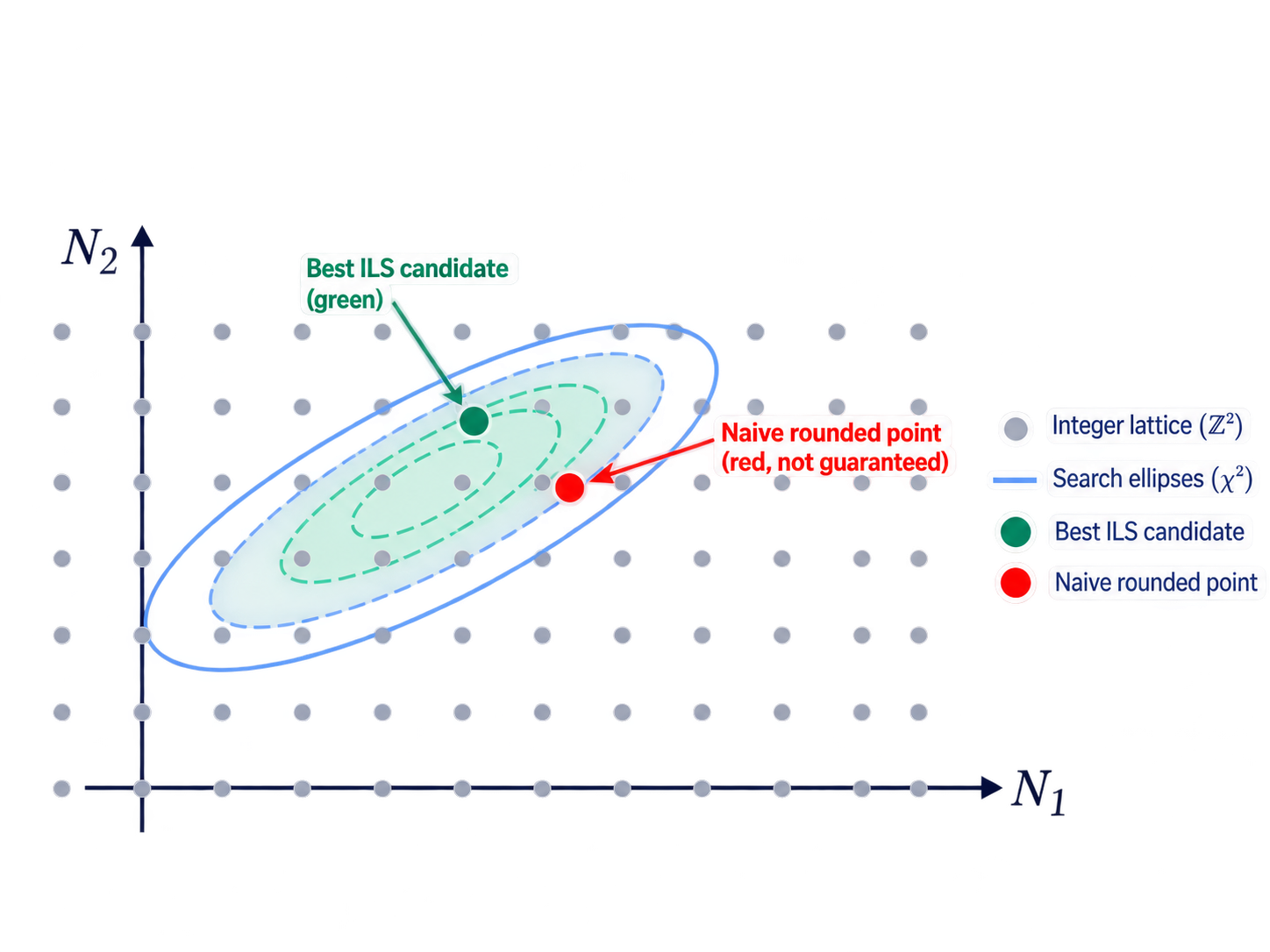
Conceptual correlated ambiguity lattice comparing an ILS candidate with naive rounding — Conceptual correlated example, not the real three-ambiguity Qelora dataset.

Why ordinary rounding can fail

Correlation tilts the distance geometry

The covariance-weighted closest point can differ from the coordinate-by-coordinate rounded point.

Keep the two examples separate

In the real three-ambiguity example below, simple rounding happens to give [1, 6, -2], the same best candidate. This 2D diagram only explains why rounding is unreliable in the general correlated case.

4. Reduction output

Read the L^T D L decomposition

These are the final reduction outputs reported by Qelora's native MLAMBDA trace for this lesson.

L=\begin{bmatrix}1&0&0\\0.333333&1&0\\0.25&0&1\end{bmatrix}

D=\begin{bmatrix}0.0808333&0&0\\0&0.06&0\\0&0&0.04\end{bmatrix}

Check the reconstruction

Q_z=L^TDL

A

Multiply D by L

D=\begin{bmatrix}0.080833&0&0\\0&0.06&0\\0&0&0.04\end{bmatrix}

x

L=\begin{bmatrix}1&0&0\\0.333333&1&0\\0.25&0&1\end{bmatrix}

=

DL=\begin{bmatrix}0.080833&0&0\\0.02&0.06&0\\0.01&0&0.04\end{bmatrix}

B

Multiply L^T by the intermediate product

L^T=\begin{bmatrix}1&0.333333&0.25\\0&1&0\\0&0&1\end{bmatrix}

x

DL=\begin{bmatrix}0.080833&0&0\\0.02&0.06&0\\0.01&0&0.04\end{bmatrix}

=

Q_z=\begin{bmatrix}0.09&0.02&0.01\\0.02&0.06&0\\0.01&0&0.04\end{bmatrix}

Interpretation: This reconstruction matches the transformed covariance for this post-reduction state. L carries triangular dependence; D carries conditional variances.

5. Integer transformation

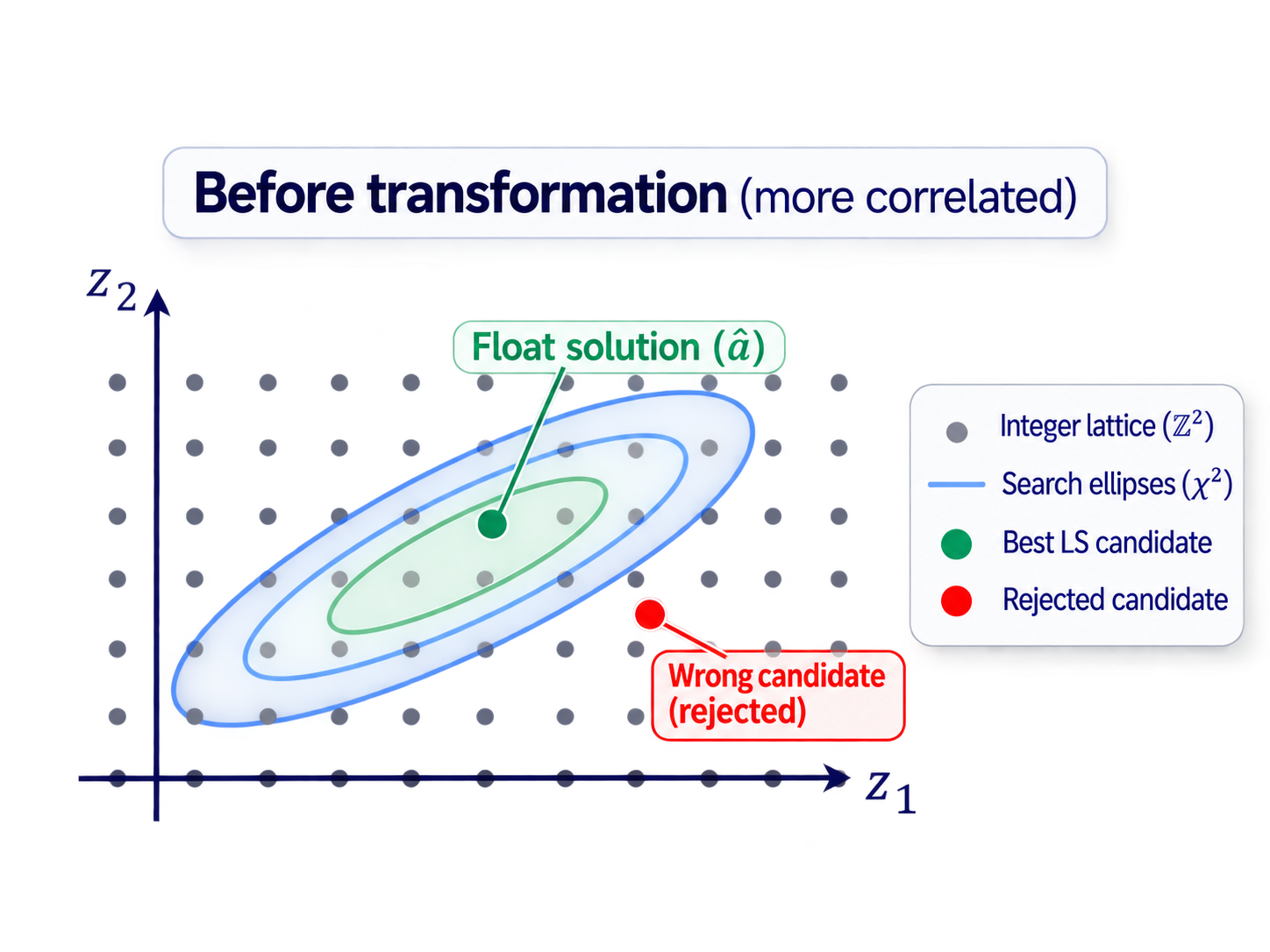
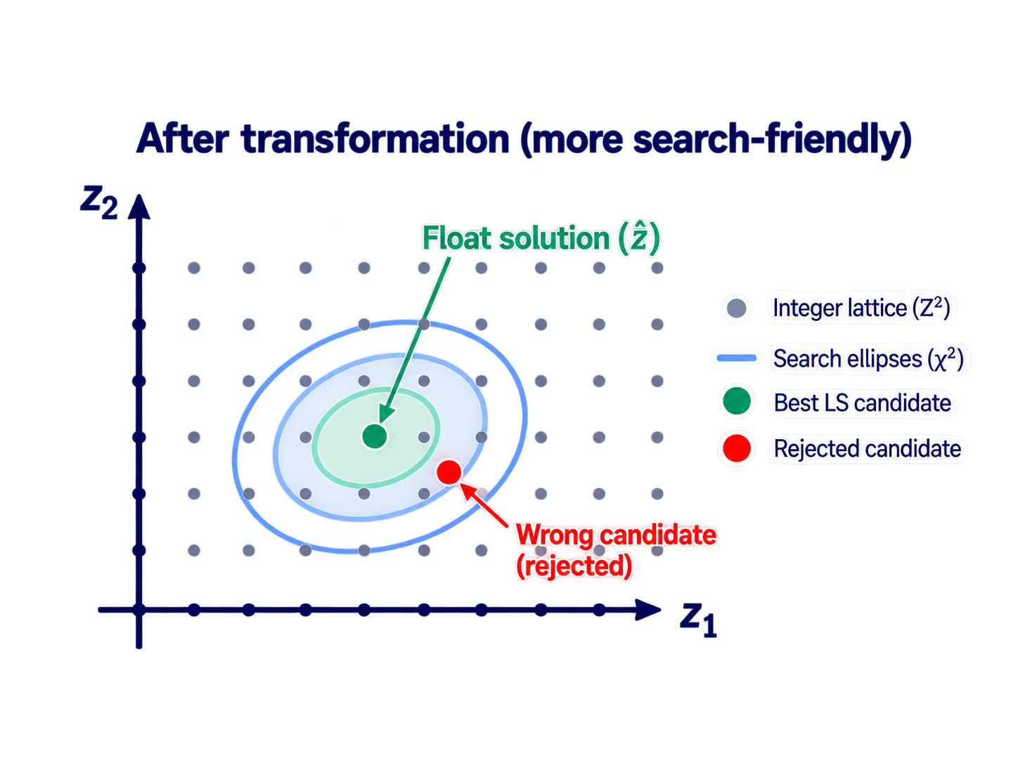
Decorrelation with the Z-transformation

Z=\begin{bmatrix}0&0&1\\1&0&0\\0&1&0\end{bmatrix}

Unimodular check

\det(Z)=+1

Every entry is an integer.
Determinant +/-1 preserves the integer lattice.
The mapping is reversible in the integer domain.

What happens in this dataset

Here Z is a permutation matrix. It mainly reorders ambiguity components, so this example does not show a dramatic decorrelation. The diagrams explain the general purpose conceptually.

Conceptual elongated correlated search ellipse before integer transformation — Conceptual: before transformation

Conceptual compact search ellipse after integer transformation — Conceptual: after transformation

6. Matrix-vector multiplication

Transform the float ambiguities

Formula

\hat{\mathbf z}=Z^T\hat{\mathbf a}

Z^T=\begin{bmatrix}0&1&0\\0&0&1\\1&0&0\end{bmatrix}

\hat{\mathbf a}=\begin{bmatrix}1.23\\5.78\\-2.41\end{bmatrix}

Row-by-row arithmetic

z_hat_1 = 0 x (1.23) + 1 x (5.78) + 0 x (-2.41) = 5.78

z_hat_2 = 0 x (1.23) + 0 x (5.78) + 1 x (-2.41) = -2.41

z_hat_3 = 1 x (1.23) + 0 x (5.78) + 0 x (-2.41) = 1.23

Result

z_hat = [5.78, -2.41, 1.23]

The values are reordered to [5.78, -2.41, 1.23]. In a more complex case, the integer transformation also reduces correlations.

7. Two-stage matrix multiplication

Transform the covariance matrix

Formula

Q_z=Z^TQ_{aa}Z

1

Compute the intermediate matrix M = Z^T Qaa

Z^T=\begin{bmatrix}0&1&0\\0&0&1\\1&0&0\end{bmatrix}

x

Q_aa=\begin{bmatrix}0.04&0.01&0\\0.01&0.09&0.02\\0&0.02&0.06\end{bmatrix}

=

M=\begin{bmatrix}0.01&0.09&0.02\\0&0.02&0.06\\0.04&0.01&0\end{bmatrix}

2

Multiply M by Z

M=\begin{bmatrix}0.01&0.09&0.02\\0&0.02&0.06\\0.04&0.01&0\end{bmatrix}

x

Z=\begin{bmatrix}0&0&1\\1&0&0\\0&1&0\end{bmatrix}

=

Q_z=\begin{bmatrix}0.09&0.02&0.01\\0.02&0.06&0\\0.01&0&0.04\end{bmatrix}

Result

Qz is the reordered covariance

Because Z is a permutation in this particular lesson, Qz largely reorders Qaa. General LAMBDA reductions can produce a much more search-friendly covariance.

8. Ellipsoidal search

Search in decorrelated z-space

1

Best candidate

z1 = [6, -2, 1]

Squared norm: 4.369536082474228

2

Second-best candidate

z2 = [6, -3, 1]

Squared norm: 9.905618556701022

Interpretation: The search evaluates integer lattice points under the covariance-weighted metric. The second candidate is valid as a candidate; it simply receives a worse score.

Conceptual integer lattice and covariance-weighted ambiguity search ellipse — Conceptual search geometry; the numerical candidates at left come from the real Qelora trace.

9. Return to original ambiguity order

Back-transform both candidates

1

Candidate 1

\mathbf n_1=Z\mathbf z_1

n_1,1 = 0 x (6) + 0 x (-2) + 1 x (1) = 1

n_1,2 = 1 x (6) + 0 x (-2) + 0 x (1) = 6

n_1,3 = 0 x (6) + 1 x (-2) + 0 x (1) = -2

Best candidate

n1 = [1, 6, -2]

The permutation restores the candidate to the original ambiguity ordering.

2

Candidate 2

\mathbf n_2=Z\mathbf z_2

n_2,1 = 0 x (6) + 0 x (-3) + 1 x (1) = 1

n_2,2 = 1 x (6) + 0 x (-3) + 0 x (1) = 6

n_2,3 = 0 x (6) + 1 x (-3) + 0 x (1) = -3

Second candidate

n2 = [1, 6, -3]

The permutation restores the candidate to the original ambiguity ordering.

10. Candidate ranking

Compute both squared norms step by step

Weighted squared distance

s_i=(\hat{\mathbf a}-\mathbf n_i)^TQ_{aa}^{-1}(\hat{\mathbf a}-\mathbf n_i)

Covariance inverse used by both calculations

Q_{aa}^{-1}=\begin{bmatrix}25.773196&-3.092784&1.030928\\-3.092784&12.371134&-4.123711\\1.030928&-4.123711&18.041237\end{bmatrix}

Candidate 1: n1 = [1, 6, -2]

1

Compute d1 = a_hat - n1

=\begin{bmatrix}1.23\\5.78\\-2.41\end{bmatrix}

-

=\begin{bmatrix}1\\6\\-2\end{bmatrix}

=

d=\begin{bmatrix}0.23\\-0.22\\-0.41\end{bmatrix}

2

Compute u1 = Qaa^-1 d1

Q_{aa}^{-1}=\begin{bmatrix}25.7732&-3.0928&1.0309\\-3.0928&12.3711&-4.1237\\1.0309&-4.1237&18.0412\end{bmatrix}

x

d=\begin{bmatrix}0.23\\-0.22\\-0.41\end{bmatrix}

=

u=\begin{bmatrix}6.185567\\-1.742268\\-6.252577\end{bmatrix}

3

Compute s1 = d1^T u1

(0.23 x 6.185567) + (-0.22 x -1.742268) + (-0.41 x -6.252577) = 4.369536082474228

Smaller score / best

s1 = 4.369536082474228

This candidate fits the float estimate and covariance model better.

Candidate 2: n2 = [1, 6, -3]

1

Compute d2 = a_hat - n2

=\begin{bmatrix}1.23\\5.78\\-2.41\end{bmatrix}

-

=\begin{bmatrix}1\\6\\-3\end{bmatrix}

=

d=\begin{bmatrix}0.23\\-0.22\\0.59\end{bmatrix}

2

Compute u2 = Qaa^-1 d2

Q_{aa}^{-1}=\begin{bmatrix}25.7732&-3.0928&1.0309\\-3.0928&12.3711&-4.1237\\1.0309&-4.1237&18.0412\end{bmatrix}

x

d=\begin{bmatrix}0.23\\-0.22\\0.59\end{bmatrix}

=

u=\begin{bmatrix}7.216495\\-5.865979\\11.78866\end{bmatrix}

3

Compute s2 = d2^T u2

(0.23 x 7.216495) + (-0.22 x -5.865979) + (0.59 x 11.78866) = 9.905618556701022

Larger score / rejected after comparison

s2 = 9.905618556701022

This candidate remains mathematically valid, but ranks behind candidate 1.

11. Estimation is not validation

Compare candidates and interpret the ratio

Best integer candidate

n1 = [1, 6, -2]

s1 = 4.369536082474228

Rejected relative to candidate 1

n2 = [1, 6, -3]

s2 = 9.905618556701022

Ratio diagnostic

\mathrm{ratio}=\frac{s_2}{s_1}=\frac{9.905618556701022}{4.3695360824742275}=2.266972596114143

The ratio measures how much worse the second candidate scores relative to the best. It is a diagnostic, not automatic proof of an acceptable fix.

Formatted ratio

2.27

Full precision: 2.266972596114143

LAMBDA estimation and ambiguity validation are separate stages

LAMBDA identifies integer candidates. Acceptance requires a chosen validation policy and may include the ratio diagnostic, residual behavior, success or failure-rate criteria, application requirements, and other quality controls. There is no single universal ratio threshold that should be hardcoded for every GNSS scenario.

12. Start-to-finish checkpoint

Complete worked numerical example

1

Input

a_hat = [1.23, 5.78, -2.41]

2

Reduction

L, D, and unimodular Z from native MLAMBDA

3

Transform

z_hat = [5.78, -2.41, 1.23]

4

Search

z1 = [6, -2, 1], z2 = [6, -3, 1]

5

Back-transform

n1 = [1, 6, -2], n2 = [1, 6, -3]

6

Metric

s1 = 4.369536, s2 = 9.905619

7

Diagnostic

ratio = 2.266972596114143

Estimator result

[1, 6, -2]

Best integer candidate from the LAMBDA estimator, not an unconditional validated fix.

13. Real Qelora implementation

Theory and production kernel

Theory

P.J.G. Teunissen's LAMBDA method provides the integer least-squares and ambiguity decorrelation foundation.

Practical implementation

Qelora uses a local native kernel compatible with the RTKLIB-style MLAMBDA implementation.

Trace consistency

api_matches_native_trace = true

The public API returned the same candidates, norms, and Z matrix exposed by the native trace.

Execution path

1

Python API

2

Input validation

3

Native MLAMBDA kernel

4

Reduction

5

Integer search

6

Back-transform

7

Candidates + metrics

result = lambda_solve(a_hat, Q_aa, n_candidates=2)
result.candidates
result.squared_norms
result.ratio

The native kernel publishes L, D, Z, z, search candidates, original-domain candidates, squared norms, and status. The tutorial does not invent unavailable internal per-line C trace details.

14. References

Theory and implementation sources

LAMBDA theory

P.J.G. Teunissen, “The least-squares ambiguity decorrelation adjustment: a method for fast GPS integer ambiguity estimation,” Journal of Geodesy, 1995.

Read the original LAMBDA paper

Qelora implementation

The practical solver is an RTKLIB-style MLAMBDA native kernel wrapped by Qelora's Python API. It is compatible with that implementation family, not claimed as a line-by-line rendering of the 1995 paper.

MLAMBDA author’s resources RTKLIB ambiguity solver source

15. What to remember

The estimator is complete; validation is the next decision

Carrier-phase ambiguities are integers, while least squares first gives float estimates.
Covariance describes both precision and dependence.
LAMBDA solves a covariance-weighted integer least-squares problem.
An integer unimodular Z transformation preserves the lattice while making search easier.
Candidates are searched in z-space and transformed back to the original ambiguity order.
Squared norms rank candidates; validation decides whether a fix is safe to use.

GNSS receiver tracking carrier-phase signals from four satellites — Integer ambiguities connect carrier-phase measurements to precise positioning.

LAMBDA Method

What does the LAMBDA method do?

Numbers before abstraction

What LAMBDA solves

Why ambiguity fixing matters

Float ambiguities and their covariance

Float ambiguity vector

Covariance matrix

The integer least-squares problem

Read the L^T D L decomposition

Check the reconstruction

Decorrelation with the Z-transformation

Transform the float ambiguities

Row-by-row arithmetic

Transform the covariance matrix

Search in decorrelated z-space

Back-transform both candidates

Candidate 1

Candidate 2

Compute both squared norms step by step

Covariance inverse used by both calculations

Candidate 1: n1 = [1, 6, -2]

Candidate 2: n2 = [1, 6, -3]

Compare candidates and interpret the ratio

Complete worked numerical example

Theory and production kernel

Execution path

Theory and implementation sources

LAMBDA theory

Qelora implementation

The estimator is complete; validation is the next decision

Double Difference

DOP Calculation

Numerical Methodology

Questions this example answers

Primary sources and further reading

Continue with the numbers